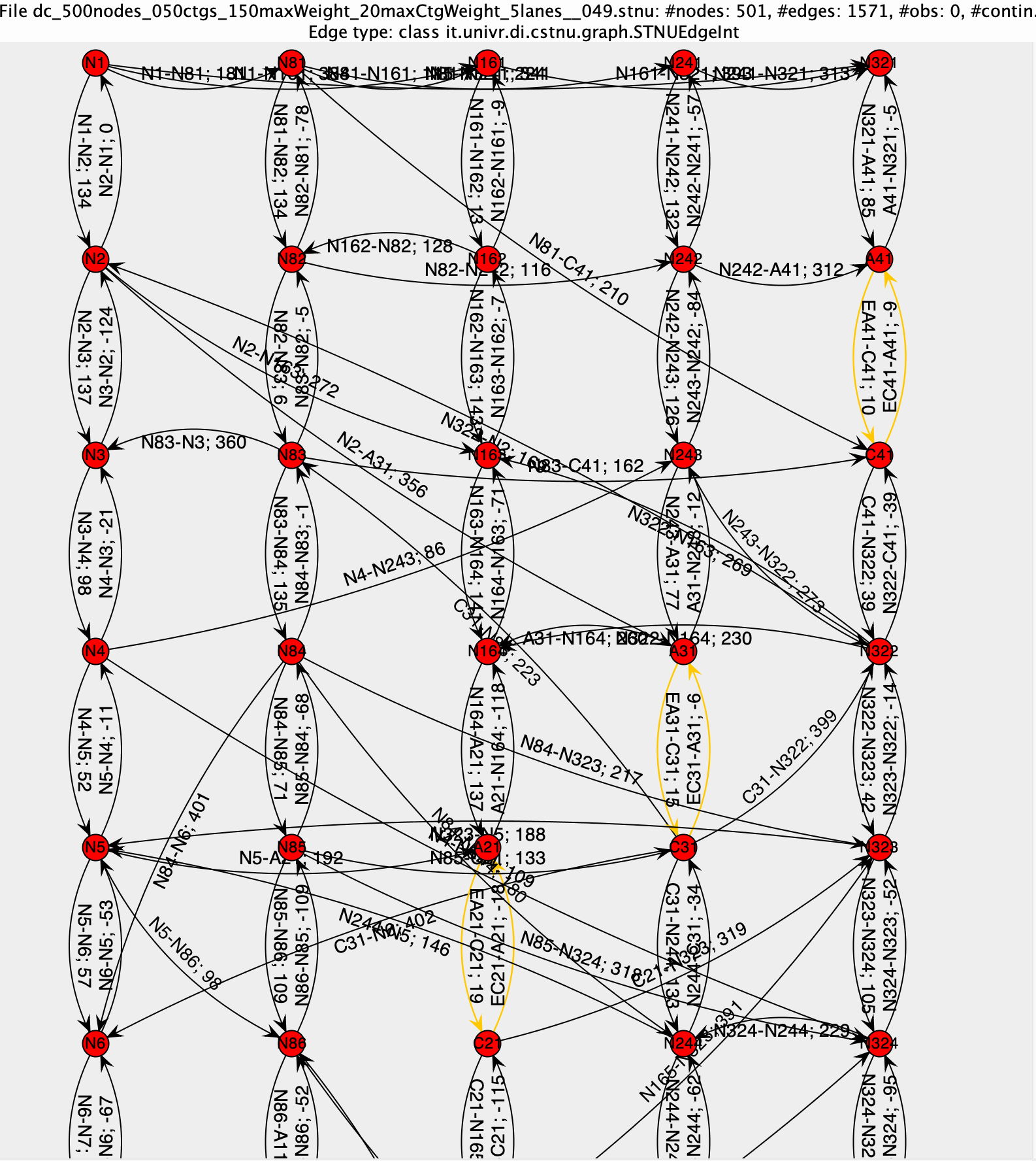
Figure 1: An example of a randomly generated STNU
The original version of this document can be downloaded at http://profs.scienze.univr.it/~posenato/software/cstnu/tex/benchmarks.pdf
During our research on temporal networks, we prepared several benchmarks for testing algorithms:
CSTNBenchmark2016 and CSTNBenchmark2018: for testing Dynamic Consistency (DC) checking algorithms for Conditional Simple Temporal Networks (CSTNs).
CSTNUBenchmark2018: for testing Dynamic Controllability (DC) checking algorithms for Conditional Simple Temporal Networks with Uncertainty (CSTNUs).
STNUBenchmark2020: for testing DC checking algorithms for Simple Temporal Networks with Uncertainty (STNUs).
CSTNPSUBenchmarks2023: for testing DC checking algorithm and Prototypal Link algorithm for Conditional Simple Temporal Networks with Partially Shrinkable Uncertainty (CSTNPSUs) (a.k.a. FTNUs).
OSTNUBenchmarks2024: for testing Agile Controllability algorithm for Simple Temporal Networks with Uncertainty and Oracles (OSTNUs).
STNUw4DiamondsBenchmark2026, STNUw6DiamondsBenchmark2026 and their two companions STNUw4DiamondsBenchmark2026WithSRCycles and STNUw6DiamondsBenchmark2026WithSRCycles: for testing algorithms that convert a dispatchable STNU into an equivalent one having a minimal number of edges, on instances that contain a nested diamond structure, without and with semi-rigid cycles. They replace STNUw4DiamondsBenchmark2025 and STNUw6DiamondsBenchmark2025, which are obsolete and are no longer distributed (Section 2.7).
CSTNBenchmark2016 and CSTNBenchmark2018 contain CSTN instances, CSTNUBenchmark2018 contains CSTNU instances, STNUBenchmark2020 contains STNU instances, CSTNPSUBenchmarks2023 contains CSTNPSU instances, and OSTNUBenchmarks2024 contains OSTNU instances. The four STNUw4Diamonds/STNUw6Diamonds archives of 2026 contain STNU instances.
All CSTN/CSTNU/CSTNPSU instances were obtained by transforming random workflows generated by the ATAPI Toolset [1], while STNU instances were obtained using the ad-hoc random generator in the CSTN Tool library.
We considered a random workflow generator as a source of random CSTN((PS)U) instances to obtain a closer approximation to real-world instances and to generate networks that are more difficult to check than those created haphazardly.
The ATAPI toolset produces random workflows according to different input parameters that govern the number of tasks, the probability of having parallel (AND)/alternative (XOR) branches, the probability of inter-task temporal constraints, and so on. In particular, the ATAPIS toolset builds a workflow instance in two phases. In the first phase, it recursively prepares the structure of the network starting from a pool of blocks representing tasks. At each cycle, it randomly removes two blocks from the pool and randomly decides how to combine them using an AND/XOR/SEQUENTIAL connector. The resulting block is then added to the pool. The generation phase ends when there is only one block in the pool. The probability of choosing an AND or an XOR connector can be given as input ( and parameters). Temporal constraints are added in the second phase according to parameters that can be given as input. The following parameter values were determined after experiments in which we tried to find a good mix that guarantees non-trivial consistent/inconsistent instances. The chosen values were:
each task duration is a subrange of ; each bound is chosen according to a beta distribution;
each connector duration always has range ;
each delay between sequential tasks is a subrange of ; each bound is chosen according to a beta distribution;
each delay between a connector and a task is fixed to ;
the probability of having an inter-activity temporal constraint between any pair of activities (i.e., tasks or connectors) was set to . When an inter-activity temporal constraint is set, its range is a random subrange of the between the two activities, where min and max distances were calculated by the tool.
For generating CSTN instances, the method consisted of two phases:
With the above parameters fixed, workflow graphs were randomly generated by varying the number of tasks (), the probability of parallel branches (), and the probability of alternative branches () to determine different blocks of instances;
each workflow graph was then translated into an equivalent CSTN using the method proposed in [2]. Task durations were represented as ordinary constraints in CSTN instances.
For generating the CSTNU instances, the method used was similar to the one above for CSTN benchmarks. The only difference was that all task durations were translated as contingent links in the corresponding CSTNU instances.
For generating the CSTNPSU instances, we considered the CSTNU instances and transformed each contingent link into a guarded one by adding the two external bounds to the contingent core. After some trials, we found that it was sufficient to enlarge the contingent core by about 10% to obtain a suitable guarded range.
During the study of DC checking algorithms for STNUs, we wanted to test the different polynomial-time algorithms using instances of significant size, i.e., much larger than the instances obtained in previous benchmarks for CSTNs or CSTNUs. We verified that increasing the size of random workflow instances built using the ATAPI toolset to obtain larger STNU instances did not work because, due to the characteristics of the generated workflows, the obtained instances were almost never DC and the generation of a few DC instances required a lot of computation.
Therefore, we decided to build a specific STNU random generator (it.univr.di.cstnu.util.STNURandomGenerator) capable of building large STNU instances. Our STNU generator can build random instances with a chosen topology that can be tuned by a variety of input parameters. The possible topologies are 1) no-topology, 2) tree, or 3) worker-lanes. After some testing, we verified that the worker-lanes topology, which simulates the swimming pools (with one lane each) of business process modeling [3], is the most interesting because it allows the generation of large random instances where there could be circuits involving many constraints. In this topology, the set of contingent links is partitioned into a given number of lanes. Contingent links within each lane are interspersed with ordinary constraints that specify delays between the end of one contingent link and the start of the next. Finally, there are constraints between pairs of nodes belonging to different lanes to represent temporal-coordination constraints among timepoints of different swimming pools. Typically, these constraints involve nodes on different lanes that are at a similar distance from the start of their respective lanes.
As an example, Figure 1 depicts a portion of a random STNU having 500 nodes and 50 contingent links in a 5-worker-lane topology.
Figure 1: An example of a randomly generated STNU
Many aspects of the worker-lanes topology can be tuned as input parameters; the number of nodes, the number of contingent links, the number of lanes, the probability of a temporal constraint for a pair of nodes from different lanes, the maximum weight of each contingent link, the maximum weight of each ordinary constraint, and so on.
This benchmark is composed of four sub-benchmarks (called benchmarks in papers [4, 5, 6, 7, 8, 9]). Each sub-benchmark is composed of two sets: one set of DC CSTN instances and one set of NOT DC instances.
Each sub-benchmark, characterized by a number , is called Size and contains CSTN instances (DC/NOT DC) generated by random workflows having tasks, XOR connectors (= propositions in CSTN), and a variable number of AND connectors. The probability of parallel branches was fixed to 0.2, as was the probability of alternative branches .
The following table summarizes the main characteristics of all sub-benchmarks:
| benchmark: | size10 | size20 | size30 | size40 |
| #tasks: | 10 | 20 | 30 | 40 |
| =#XOR: | 3 | 5 | 7 | 9 |
| #CSTN-nodes: | 45-59 | 79-95 | 123-135 | 159-175 |
For each sub-benchmark, there are at least 60 dynamically consistent CSTNs and 20 non-dynamically consistent CSTNs. Since the original ATAPIS toolset allows the user to fix only the probability of AND/XOR connectors, it was necessary to run the toolset a huge number of times to obtain the instances with the above characteristics.
Different workflow graphs with the same number of tasks may translate into CSTNs of different sizes because of different numbers of AND connectors in the workflows. This fact represented the main weakness of this benchmark. For example, even if for and there are 60 DC instances, these instances are CSTN instances with different orders (=#nodes). Few of them have the same order, and this fact represents a limitation when an evaluation of DC execution time with respect to the CSTN order is required.
For this benchmark, we do not report here the results obtained using our algorithms because they are superseded by the results obtained with CSTNBenchmark2018, presented in the next section.
The structure of this benchmark is equal to that of CSTNBenchmark2016: four sub-benchmarks with two sets for each. The main differences are the number of instances and the structure of the instances.
After an important modification of the ATAPI Toolset source code, it was also possible to give as input the number of XOR/AND connectors that a random workflow instance must have. Therefore, it was possible to build sets of more uniform instances where randomness could decide how to mix components and constraints, but not their quantities. It is possible to show that the relation between workflow component quantities and CSTN order is , where is the number of tasks, the number of XOR connectors, and the number of AND connectors. Therefore, for each planned combination of #task-#XOR-#AND, it was possible to randomly generate 50 DC and 50 NOT DC instances. The following table summarizes the characteristics of each sub-benchmark.
| Group | Benchmark | instance indexes | # activities | #XOR | #AND | CSTN order |
| Size010-3 | B10-3-0 | 000-049 | 10 | 3 | 0 | 43 |
| B10-3-1 | 050-099 | 10 | 3 | 1 | 47 |
|
| B10-3-2 | 100-149 | 10 | 3 | 2 | 51 | |
| B10-3-3 | 150-199 | 10 | 3 | 3 | 55 |
|
| B10-3-4 | 200-249 | 10 | 3 | 4 | 59 | |
| Size020-5 | B20-5-0 | 000-029 | 20 | 5 | 0 | 75 |
| B20-5-1 | 030-059 | 20 | 5 | 1 | 79 | |
| B20-5-2 | 060-099 | 20 | 5 | 2 | 83 |
|
| B20-5-3 | 090-119 | 20 | 5 | 3 | 87 |
|
| B20-5-4 | 120-149 | 20 | 5 | 4 | 91 |
|
| Size030-7 | B30-7-0 | 000-029 | 30 | 7 | 0 | 107 |
| B30-7-1 | 030-059 | 30 | 7 | 1 | 111 |
|
| B30-7-2 | 060-089 | 30 | 7 | 2 | 115 |
|
| B30-7-3 | 090-119 | 30 | 7 | 3 | 119 |
|
| B30-7-4 | 120-149 | 30 | 7 | 4 | 123 |
|
| Size040-9 | B40-9-0 | 000-029 | 40 | 9 | 0 | 139 |
| B40-9-1 | 030-059 | 40 | 9 | 1 | 143 |
|
| B40-9-2 | 060-089 | 40 | 9 | 2 | 147 |
|
| B40-9-3 | 090-119 | 40 | 9 | 3 | 151 |
|
| B40-9-4 | 120-149 | 40 | 9 | 4 | 155 |
|
The total number of CSTN instances is , DC and NOT DC, divided into 4 main groups, in turn divided into 4 other groups having 50 DC and 50 NOT DC instances.
We used CSTNBenchmark2018 for testing 10 different DC checking algorithms for CSTNs:
In the following, we present two diagrams that compare these algorithms using the CSTNBenchmark2018 benchmark.
We executed the algorithm implementations in the CSTNU Tool library using an Oracle JVM 8 on a Linux machine with an AMD Opteron 4334 CPU (12 cores) and 64GB of RAM.
The execution times were collected by a Java program (Checker, present in CSTNU Tool) that allows the user to determine the average execution time—and its standard deviation—of one DC checking algorithm applied to a set of CSTN instances. We observed that even though the AMD Opteron 4334 has 12 cores, the best performance was obtained only when all checks were made by only one core. We verified that memory access by cores represents a bottleneck that limits the overall performance. Therefore, all the data presented in this section were obtained sequentially, with one check at a time.
The parameters for the Oracle Java Virtual Machine 1.8.0_144 were: -d64, -Xmx6g, -Xms6g, -XX:NewSize=3g, -XX:MaxNewSize=3g, -XX:+UseG1GC, -Xnoclassgc, and -XX:+AggressiveOpts.
The first diagram shows the average execution times of all algorithms with respect to the order of dynamically consistent CSTN instances. Each drawn value is the sample average of execution times obtained considering the fifty instances of the relative benchmark. In detail, where is the average execution time obtained by executing the algorithm 3 times on the instance having index 1. The error bar of each drawn value represents times the standard error of the mean, , where is the corrected sample standard deviation, . The value is the Student’s distribution value with 49 degrees of freedom. Therefore, the error bar represents a 95% confidence interval for the average execution time of the algorithm on instances having the main characteristics of the considered benchmark.
![[Picture]](images/benchmarks0x.svg)
Although the diagram is quite crowded, it is possible to see (and data confirm) that the DC checking algorithm has the worst performance when it has to apply IR semantics without node labels while the fastest DC checking can be done using the Potential algorithm. The outstanding performance of Potential algorithm can be justified observing that this algorithm does not add constraints to the network but only potential values to nodes and that the quantity of such values is, in general, lower than the number of new constraints added by other algorithms.
We noted that the experimental data contain outliers, instances for which the execution time is quite far from the average execution time. Outliers represent hard instances for the DC checking problem (the problem was shown to be PSPACE-complete).
The following figures show the distribution of execution time of IR-3R in terms of quartiles in the groups Size030-7 and Size040-9. Each box has the lower edge equal to the first quartile () while the upper edge equal to the third one (). The edge inside each box represents the median of the sample. Horizontal edges outside a box represent the whiskers. The lower whisker value is the smallest data value which is larger than , where IQR is the inter–quartile–range, i.e., . The upper whisker is the largest data value which is smaller than . Diamonds above the upper whisker represent the data value outliers. The diamond in the highest position in each set of data represents the worst case value of the benchmark. Diamond inside a box represents the average value of the benchmark.
![[Picture]](images/benchmarks1x.svg)
![[Picture]](images/benchmarks2x.svg)
The previous two diagrams show clearly that there are few instances that bias the value of sample average in a relevant way.
The following diagram shows the average execution times of some checking algorithms when CSTN instances are inconsistent.
![[Picture]](images/benchmarks3x.svg)
Again, even if the diagram is quite crowded, it is evident that Std-woNL shows the worst performance while IR-3R requires the minimum execution time for almost of the group of instances. Algorithm Potential has not an outstanding performance like for DC instances because the presence of negative circuits is, in general, determined promptly and, therefore, the execution time cannot be different significantly. The most important fact about these results is that, in general, checking NON DC instances requires less than an order of magnitude of execution time required for checking DC instances.
This benchmark was used for testing the algorithms that check the dynamic controllability of CSTNUs [10].
The structure of this benchmark is similar to the CSTNBenchmark2018 one with two differences: the duration of each task is converted as contingent link and the number of instances is smaller.
Due to the internal building function of ATAPIS Toolset, the relation between workflow component quantities and CSTNU order is , where is the number of tasks, the number of XOR connectors, and the number of AND connectors. The following table summarizes the characteristics of each sub-benchmark.
| Group | Benchmark | instance indexes | #tasks | #XOR | #AND | CSTNU order |
| Size010-3 | B10-3-0 | 000-049 | 10 | 3 | 0 | 43 |
| B10-3-1 | 050-099 | 10 | 3 | 1 | 49 |
|
| B10-3-2 | 100-149 | 10 | 3 | 2 | 55 | |
| B10-3-3 | 150-199 | 10 | 3 | 3 | 61 |
|
| B10-3-4 | 200-249 | 10 | 3 | 4 | 67 | |
| Size010-4 | B10-4-0 | 000-049 | 10 | 4 | 0 | 49 |
| B10-4-1 | 050-099 | 10 | 4 | 1 | 55 |
|
| B10-4-2 | 100-149 | 10 | 4 | 2 | 61 |
|
| B10-4-3 | 150-199 | 10 | 4 | 3 | 67 |
|
| B10-4-4 | 200-249 | 10 | 4 | 4 | 73 |
|
| Size010-5 | B10-5-0 | 000-049 | 10 | 5 | 0 | 55 |
| B10-5-1 | 050-099 | 10 | 5 | 1 | 62 |
|
| B10-5-2 | 100-149 | 10 | 5 | 2 | 67 |
|
| B10-5-3 | 150-199 | 10 | 5 | 3 | 73 |
|
| B10-5-4 | 200-249 | 10 | 5 | 4 | 79 |
|
The total number of CSTNU instances is , DC and NOT DC, divided into 3 main groups—Size010-3, Size010-4, and Size010-5—in turn divided into 5 other groups having 50 DC instances each and 5 other groups having 50 NOT DC instances each.
There are three implementations of the CSTNU DC checking algorithm:
In the following, we present some diagrams that show the execution times of all versions in the CSTNUBenchmark2018 benchmark.
The implementations were developed in Java 8 and run on an Oracle JVM 8 on a Linux machine with an Intel(R) Xeon(R) CPU E5-2637 v4 3.50GHz and 503GB of RAM.
The execution times were collected by a Java program (Checker, included in our package) that allows the user to determine the average execution time—and its standard deviation—of a DC checking algorithm applied to a set of instances.
The parameters for the Oracle Java Virtual Machine 1.8.0_144 were: -d64, -Xmx6g, -Xms6g, -XX:NewSize=3g, -XX:MaxNewSize=3g, -XX:+UseG1GC, -Xnoclassgc, and -XX:+AggressiveOpts.
All average execution times were determined considering only DC instances in benchmarks of groups Size010-3, Size010-4, and Size010-5. Each drawn value is the sample average of execution times obtained considering fifty instances of the relative benchmark. In detail, where is the average execution time obtained by executing the algorithm 3 times on the instance having index 2. The error bar of each drawn value represents times the standard error of the mean, , where is the corrected sample standard deviation, . The value is the Student’s distribution value with 49 degrees of freedom. Therefore, the error bar represents a 95% confidence interval for the average execution time of the algorithm on instances of the considered benchmark.
In more detail, Figure 6 shows the performance of the three implementations in benchmarks of group Size010-3. Each printed value corresponds to the average value determined considering the corresponding sub-benchmark B10-3-*. We observed some run time-outs (45 minutes) for the STD and STD OnlyToZ algorithms. The average execution time was determined by also considering these time-outs and, therefore, it represents a lower bound to the real average.
All three implementations require, on average, a smaller execution time as the order of instances increases. This is due to the fact that the bigger instances are obtained by increasing the number of parallel connectors in the generated workflows (the number of contingent links and the number of observation nodes are fixed). Increasing the number of parallel connectors creates more parallel branches and, therefore, more contingent links must be put in the same scenario. This makes a network easier to check.
From the experimental results, it emerges that CSTNU2CSTN has the best performance and the worst performance for all implementations is in the sub-benchmark B10-*-0, where all generated workflows have no parallel branches.
![[Picture]](images/benchmarks4x.svg)
Figure 7 shows a detail about the worst-case execution time. For each sub-benchmark Size10-*-0, i.e., instances derived by workflows without parallel flows, we report the average execution time to show how the average execution time increases as the number of choices increases.
![[Picture]](images/benchmarks5x.svg)
Again, it is clear that the CSTNU2CSTN has the best performance.
Figure 8 shows the average execution time obtained when instances are not DC. The algorithms have worse performance when checking non-DC instances than when checking DC ones. On average, each algorithm requires an average execution time that can be 8 times greater than the average execution time required for checking positive instances having the same order.
![[Picture]](images/benchmarks6x.svg)
This benchmark is composed of five sub-benchmarks (named as Test 1 benchmarks in [11]). Each sub-benchmark is composed of two sets: one set of DC STNU instances and one set of non-DC ones.
Each sub-benchmark, characterized by a number
,
contains STNU instances (DC/NOT DC) generated randomly using
it.univr.di.cstnu.util.STNURandomGenerator (see Section 1.2) with the following
parameters
|
| |
|
|
|
| Number of nodes, |
|
|
| |
|
|
|
| Number of lanes | 5 |
|
|
|
|
|
|
| Number of contingent links, | (hence, ) |
|
|
|
|
|
|
| Max absolute weight of ordinary edges | 150 |
|
|
|
|
|
|
| Max contingent range |
|
|
|
|
|
|
|
| Probability of constraint among nodes in different lanes | 0.40 |
|
|
|
|
|
|
For these parameter choices, each node (except the first and the last one of each lane) has two incoming edges and two outgoing edges in the same lane, as well as an average of incident edges representing temporal-coordination constraints with nodes in other lanes. Activation timepoints have no temporal constraint with nodes of other lanes because we preferred to derive them from the constraints incident to their contingent timepoints. Temporal-coordination constraints are set in a way that avoids introducing negative circuits among a pair of nodes. Therefore, the number of edges is, on average, ; hence, . For each value of , the benchmark contains 200 DC networks and 200 non-DC networks for a total of 2000 instances distributed in ten sub-benchmarks.
Moreover, in each sub-benchmark of DC instances there are 100 instances that are copies of the first DC instances of the benchmark but where the number of contingent links is reduced to .
In the CSTNU Tool library, there are three different STNU DC checking algorithms:
All these implementations are available as DC checking options in the class it.univr.di.cstnu.algorithms.STNU in CSTNU Tool library.
In the following, we present two diagrams that show the performance of the three algorithms using the STNUBenchmark2020 benchmark.
We used an Oracle JVM 8 having 8GB of heap memory on a Linux box with one Intel(R) Xeon(R) CPU E5-2637 v4 @ 3.50GHz. The parameters for the Oracle Java Virtual Machine 1.8.0_144 were: -Xmx8g, and -Xms8g.
The execution times were collected by a Java program (Checker, included in our package) that allows the user to determine the average execution time—and its standard deviation—of a DC checking algorithm applied to a set of instances.
Figures 9 and 10 display the average execution times of the three algorithms across all ten sub-benchmarks.
![[Picture]](images/benchmarks7x.svg)
![[Picture]](images/benchmarks8x.svg)
Each plotted point represents average execution time over 200 instances
Each plotted point represents the average execution time for a given algorithm on the 200 instances of the given size, and the error bar for each point represents the 95% confidence interval. For example, over the 200 DC instances having timepoints and contingent links, the average execution time (in seconds) of the Morris14algorithm lies within the interval with 95% confidence, while the average execution time of the RUL20algorithm lies within the interval with 95% of confidence. These results demonstrate that the RUL20algorithm performs significantly better than the other two algorithms, especially over DC instances, but also over non-DC instances. For non-DC instances, the 95%-confidence intervals tend to be larger than those for the corresponding DC instances because for some non-DC instances the negative cycle can be detected immediately (e.g., by an initial run of Bellman-Ford or during the processing of the first contingent link or negative node), while others may require significant amounts of propagation.
One of our principal motivating hypotheses was that our new algorithm would be significantly faster than the RULalgorithm because it inserts significantly fewer new edges into the input STNU graph. In particular, whereas the RULalgorithm computes and inserts new edges arising from all three of the RULrules, the RUL20algorithm only inserts edges arising from the length-preserving case of one rule.
The structure of this benchmark is similar to that of CSTNUBenchmark2020, with two differences: the duration of each task is converted to a guarded link by adding two external bounds to the core. The external bounds enlarge the core by about 10% on each side. In particular, each contingent link was replaced by the guarded link , where was set to while was set to , where .
Since the scope of this benchmark was to check the performance of the PrototypalLink algorithm, which is significant only for DC instances, the benchmarks contain only DC instances.
The following table summarizes the characteristics of each sub-benchmark.
| Group | Benchmark | instance indexes | #tasks | #XOR | #AND | CSTNPSU order |
| Size010-3 | B10-3-0 | 000-049 | 10 | 3 | 0 | 43 |
| B10-3-1 | 050-099 | 10 | 3 | 1 | 49 |
|
| B10-3-2 | 100-149 | 10 | 3 | 2 | 55 |
|
| B10-3-3 | 150-199 | 10 | 3 | 3 | 61 |
|
| B10-3-4 | 200-249 | 10 | 3 | 4 | 67 |
|
The total number of CSTNPSU instances is DC, divided into 5 groups having 50 DC instances each.
This section presents an empirical evaluation of the performance of the FTNU DC-checking algorithm and of the getPrototypalLink procedure.
We recall that the getPrototypalLink procedure, given a DC instance as input, has to determine the completion of the instance and the path contingency span of each node to calculate the prototypal link.
The comparison of the performance of the two algorithms should give an idea of the computational cost of having a compact representation of a (sub)process versus the cost of determining only its controllability.
The tests were executed using a Java Virtual Machine 17 on an Apple PowerBook (M1 Pro processor) configured to use 8 GB memory as heap space.
Figure 11 displays the average execution times of the two algorithms over all five sub-benchmarks in B3, B4, and B5.
![[Picture]](images/benchmarks9x.svg)
Each data point value is the sample average of average execution times obtained considering the fifty instances of the relative sub-benchmark. Indeed, each is the average execution time obtained by executing the algorithm five times on the instance having index in the considered sub-benchmark. The error bar represents a 95% confidence interval for the average execution time of the algorithm on instances of the considered sub-benchmark.
As concerns the FTNU DC checking performance, from the data in Figure 11, it follows that the performance is similar to that obtained for the CSTNU DC checking algorithm in [10], although here the average times are one order of magnitude smaller (thanks to the M1 processor). The more difficult instances are associated with workflows without parallel gateways (i.e., instances in the first sub-benchmark of each main benchmark), and the algorithm performs better as the number of AND gateways increases, except in B5. As stated in [14], such behavior is due to how the ATAPIS random generator works when the number of AND gateways is small (i.e., less than 5). Increasing the number of AND gateways (up to 5), fewer XOR gateways are set in sequence and, therefore, there are fewer possible scenarios. In B, where the number of AND gateways is 4, this pattern did not occur. The sub-benchmark contains many instances with three or four observation timepoints over five in sequence, determining a greater number of possible scenarios and, hence, a greater execution time for the checking.
As concerns the getPrototypalLink procedure, its execution times are much lower than those of the DC checking algorithm (see Figure 11). Figure 12 shows the average execution time of getPrototypalLink of Figure 11 in linear -scale. Once a network is checked DC, the completion phase updates the values of the original guarded and requirement links in the network, while the building of the path contingency span graph creates and fills a vector of labeled distances from Z to each node. These phases require visiting each original edge of the network twice, each time considering all the labeled values associated with the edge. We verified that the average node degree is less than 5 in all benchmarks, hence the instances are sparse graphs. In these benchmarks, the quantity of labeled values present in each edge is not as relevant as the number of edges/nodes in determining the computation time. Therefore, the getPrototypalLink performance is quasi-linear with respect to the number of nodes.
![[Picture]](images/benchmarks10x.svg)
This benchmark is for testing the Agile Controllability (AC) checking algorithm for Simple Temporal Networks with Uncertainty and Oracles (OSTNUs), introduced in [15]. In an OSTNU, a contingent link may have an associated oracle: a timepoint that, when executed, reveals the duration the contingent link will take, so that the executor may exploit the information before the contingent timepoint occurs.
The instances were not generated from scratch: they were obtained by reducing 30 random DC instances of the DC 500 sub-benchmark of Section 2.4 — STNUs of 500 nodes and 50 contingent links representing random temporal business processes — to OSTNUs of the following shape.
|
| |
|
|
|
| Number of nodes, | 30 |
|
| |
|
|
|
| Number of lanes | 3 |
|
|
|
|
| |
| Number of contingent links, | 5 |
|
|
|
|
|
|
| Number of oracles | 2 |
|
|
|
|
|
|
| Max absolute weight of ordinary edges | 150 |
|
|
|
|
|
|
| Max contingent range |
|
|
|
|
|
|
|
The 30 instances are split into 27 AC ones and 3 non-AC ones: the AC ones are the interesting ones for evaluating the checking algorithm, hence the asymmetry. The AC instances are provided both in the GraphML format used by the CSTNU Tool (extension .ostnu) and in a plain textual format (extension .plainOStnu); the non-AC ones are provided in the GraphML format only.
On these instances, the average AC-checking time of the labeling-based algorithm of [15] is around 3 seconds. The AC checking is exponential in the number of (contingent, oracle) pairs in the worst case, which is why the instances are deliberately small: the reduction to 30 nodes with 5 contingent links and 2 oracles keeps the number of such pairs within the range the tool can manage (at most 26 pairs, for efficiency reasons).
These two archives are obsolete and are no longer distributed; Section 2.8 describes the four archives of 2026 that replace them. The reason lies in the instances themselves. The node of a diamond gadget receives the stand-in edge of every diamond of the structure and has no edge leaving it, so the structure takes constraints and propagates none, and does not constrain the rest of the network at all – the opposite of what it was introduced for. This was verified on the published files: in all their 240 instances, not one edge leaves a node named . The random generator of the tool now connects that node itself. The tables and the two figures below are kept because they document the evaluation published in [16], which was run on those instances.
These two benchmarks support the work on converting a dispatchable STNU into an equivalent one having a minimal number of edges [17, 18, 16]. The number of edges matters because a dispatchable network is executed by propagating only the constraints incident to the timepoint just executed, so the size of the network is the dominant cost at execution time.
They exist because of a negative finding: while evaluating those algorithms on Section 2.4, it turned out that no instance of that benchmark contains a nested diamond structure [19], the configuration of contingent links whose stand-in edges cannot be determined independently of one another and have to be analysed in a specific order. Without such a structure, the algorithm that generates stand-in edges by repeated all-node cycles and the one designed for many diamonds do essentially the same work, and no difference in performance can be observed. The two benchmarks were therefore created to make that difference measurable: every instance contains one copy of a nested diamond structure, of depth 4 in the first benchmark and of depth 6 in the second.
Both benchmarks were generated with it.univr.di.cstnu.util.STNURandomGenerator (see Section 1.2) with the following parameters.
|
| |
|
|
|
| Number of nodes, |
|
|
| |
|
|
|
| Number of lanes | 5 |
|
|
|
|
|
|
| Number of contingent links, |
|
|
|
|
|
|
|
| Max absolute weight of ordinary edges | 150 |
|
|
|
|
|
|
| Max contingent range |
|
|
|
|
|
|
|
| Nested diamond structure | one copy per instance, of depth 4 (w4) or depth 6 (w6) |
|
|
|
|
|
|
For each value of each benchmark contains 30 DC instances, for a total of 120 instances per benchmark. Instances are in the plain textual format (extension .plainStnu). Both benchmarks contain DC instances only, by construction: the minimization applies to a network that has been made dispatchable, and only a dynamically controllable network can be made dispatchable.
The evaluation reported in [16] was run on an OpenJDK 21 JVM configured with 16 GB of heap memory, on a Linux computer with two AMD Opteron™ 4334 processors at 3.1 GHz and 64 GB of RAM. Each DC instance was first made dispatchable by the FD algorithm, and the resulting dispatchable ESTNU was then fed to the two minimization algorithms, so that their outputs could be compared for identity and their execution times for speed.
On both benchmarks the newer algorithm is significantly faster than the older one across all instances, and for instances of 2000 nodes the older one exceeded the 30-minute timeout. The reason is visible in the two complexities: the presence of a depth-4 nested diamond makes the older stand-in generation perform up to five iterations, each taking time, whereas its replacement costs regardless of how deeply the diamond is nested.
The depth-6 benchmark was expected to widen the gap further, and it did not, for a reason worth recording: the random constraints between nodes of different lanes and nodes of the diamond structure sometimes entail constraints stronger than the stand-in edges of the diamond itself, so on average the older algorithm still performs about five internal iterations — the same number as on the depth-4 instances.
The measured execution times are in Figure 1 and Figure 2, reproduced from [16]. Note that the curve of minDispESTNUstops before the largest size: for instances of 2000 nodes its execution exceeded the 30-minute timeout.
These four archives replace the two of 2025 and serve the same purpose, on instances where the nested diamond structure is really connected to the rest of the network:
STNUw4DiamondsBenchmark2026 and STNUw6DiamondsBenchmark2026: DC instances containing one nested diamond structure, of depth 4 and of depth 6 respectively;
STNUw4DiamondsBenchmark2026WithSRCycles and STNUw6DiamondsBenchmark2026WithSRCycles: the same instances, completed with semi-rigid cycles.
All four were generated with it.univr.di.cstnu.util.STNURandomGenerator (see Section 1.2) with the following parameters.
|
| |
|
|
|
| Number of nodes, |
|
|
| |
|
|
|
| Number of lanes | 5 |
|
|
|
|
|
|
| Number of contingent links, |
|
|
| |
|
|
|
| Max node in-degree and out-degree | 20 |
|
| |
|
|
|
| Edge probability | 0.40 |
|
|
|
|
|
|
| Max absolute weight of ordinary edges | 150 |
|
|
|
|
|
|
| Max contingent weight | 20 |
|
|
|
|
|
|
| Max contingent range | 15 |
|
|
|
|
|
|
| Nested diamond structure | one copy per instance, of depth 4 (w4) or depth 6 (w6) |
|
|
|
|
|
|
For each value of each archive contains 30 DC instances, for a total of 120 instances per archive. Every instance is present both in the GraphML dialect of the tool (extension .stnu) and in the plain textual format (extension .plainStnu). All the instances are DC: the minimization applies to a network that has been made dispatchable, and only a dynamically controllable network can be made dispatchable.
A semi-rigid cycle is a cycle of the ordinary+wait graph formed by a wait edge and an ordinary path whose length is exactly the magnitude of that wait. Its two ends are then rigidly related for as long as the contingent duration behind the wait remains unobserved, and a stand-in edge closing such a cycle cannot be discarded without changing the network: this is the case that separates an algorithm which keeps those edges from one which does not. In these instances every diamond generates one wait of magnitude 3, and the completion adds, for each diamond, the single ordinary edge that makes a path from the activation time point to the source of the wait measure exactly 3. An instance whose structure has depth therefore carries semi-rigid cycles: four in the w4 archive, six in the w6 one. The edges are added by it.univr.di.cstnu.util.STNUAddSemiRigidCycles, which then restores dynamic controllability by relaxing negative ordinary constraints outside the structure, and verifies that every one of those paths is still tight before writing the instance.
The two halves match one to one: the instance of index of a WithSRCycles archive is the instance of index of the corresponding archive, with the cycle-closing edges added and the relaxation applied. A measurement can therefore be repeated on the same network with and without semi-rigid cycles.
Every instance also carries two pieces of information that the earlier benchmarks lack: the name of its own file, and the outcome of the dynamic-controllability check that accepted it – the verdict, the algorithm that established it and the version of the tool that wrote it – stored beside a fingerprint of the network. A reader can therefore trust that verdict without running a check again, while the tool itself ignores it as soon as the network is modified. The File format page of this website documents the three GraphML keys involved.
![[Picture]](images/benchmarks11x.svg)
![[Picture]](images/benchmarks12x.svg)